


Bayesian updates to multi-age Antarctic sea-ice concentrations using GNSS-R data
Speaker: Steefan Contractor
Coauthors: Shane Keating (UNSW), Jessica Cartwright (Spire Global), Alex Fraser (UTAS)
Sea Ice
- Floating ice that forms from the freezing of seawater
- Melting and formation of sea ice affects the ocean salinity and heat content
- The changes in ocean density and temperature affect the ocean circulation as evidenced by recent coverage on AMOC weakening
- It affects the Earth’s energy balance by reflecting ten times more sunlight compared to water
- It acts like a blanket affecting not just heat exchange between the ocean and atmosphere but also gases
- Through the changes in polar air masses it also affects atmospheric circulation
Image sources:
- Novel application of GNSS-R data from TechDemoSat-1 to monitoring the cryosphere, Jessica Cartwright
- https://www.ccin.ca/ccw/seaice/overview/types
- Australian Antarctic Program
- https://www.sciencefriday.com/wp-content/uploads/2017/02/fce480147c3334975973a38782f1382c-min.jpg
- https://www.youtube.com/watch?v=_iTBQiE2CuM
- https://johnenglander.net/wp/wp-content/uploads/2018/05/young-sea-ice.jpeg
- WMO Sea Ice Nomenclature WMO-No. 259
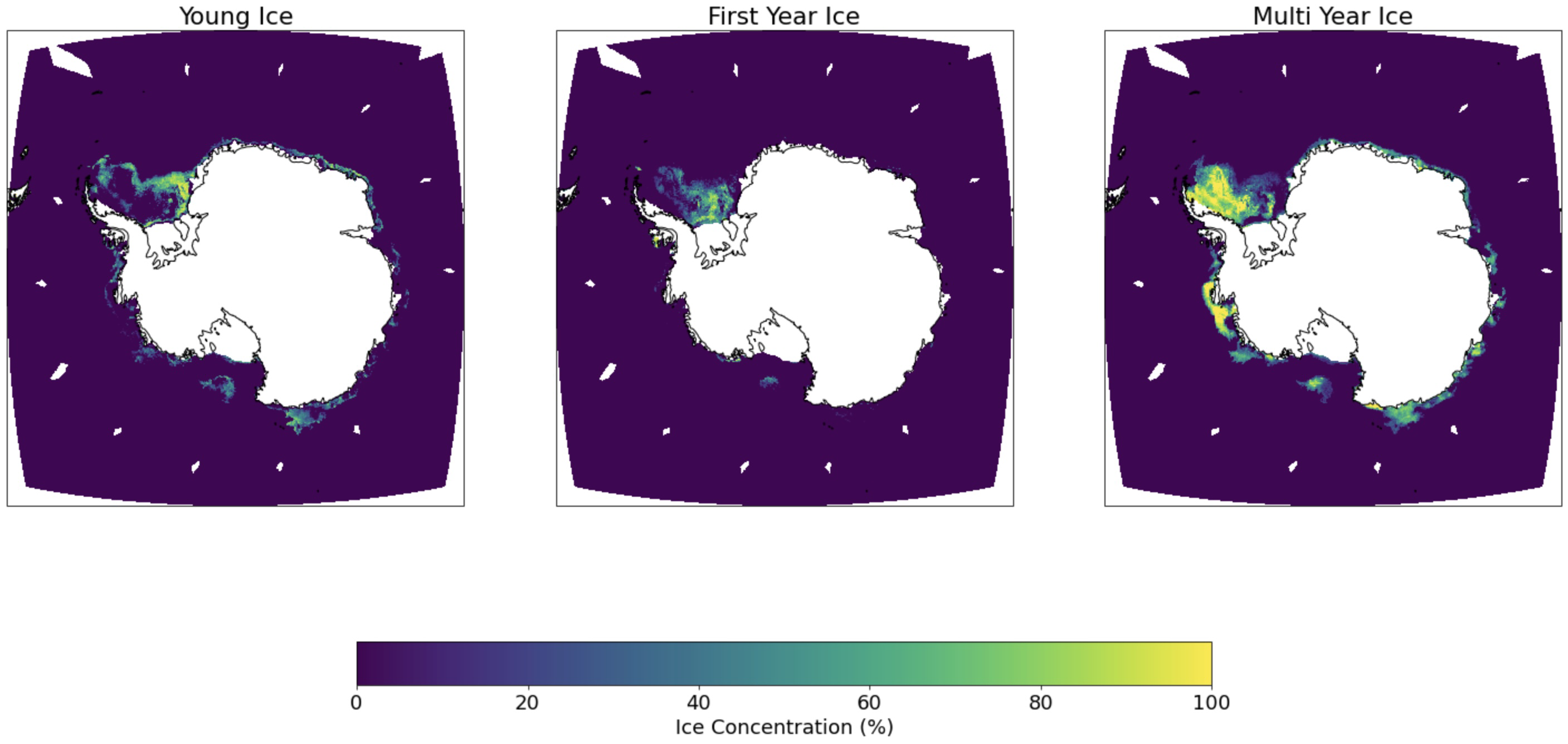
Young Ice (YI)
- Newly formed ice
- can be rough or smooth
- less than 30cm thick
First-year Ice (FYI)
- Ice that has survived one summer melt season
- can be level, rough or have ridges
- 30cm to 2m thick
Multi-year Ice (MYI)
- Ice that has survived more than one summer melt season
- typically smoother than FYI
- Over 2.5m thick and hence protrudes above the waterline
- has extremely low salinity compared to YI and FYI
Remote Sensing of Sea Ice
Active sensors
- Radar altimeters (CrysoSat-2)
- Laser altimeters (IceSat-2)
- Scatterometers (Metop A/B/C - ASCAT)
- Synthetic Aperture Radar (Radarsat-2)
Passive sensors
- Passive microwave radiometers (SMOS)
Hybrid sensors
- Global Navigation Satellite System Reflectometry - GNSS-R
IUP U. Bremen Multiage Ice Concentration
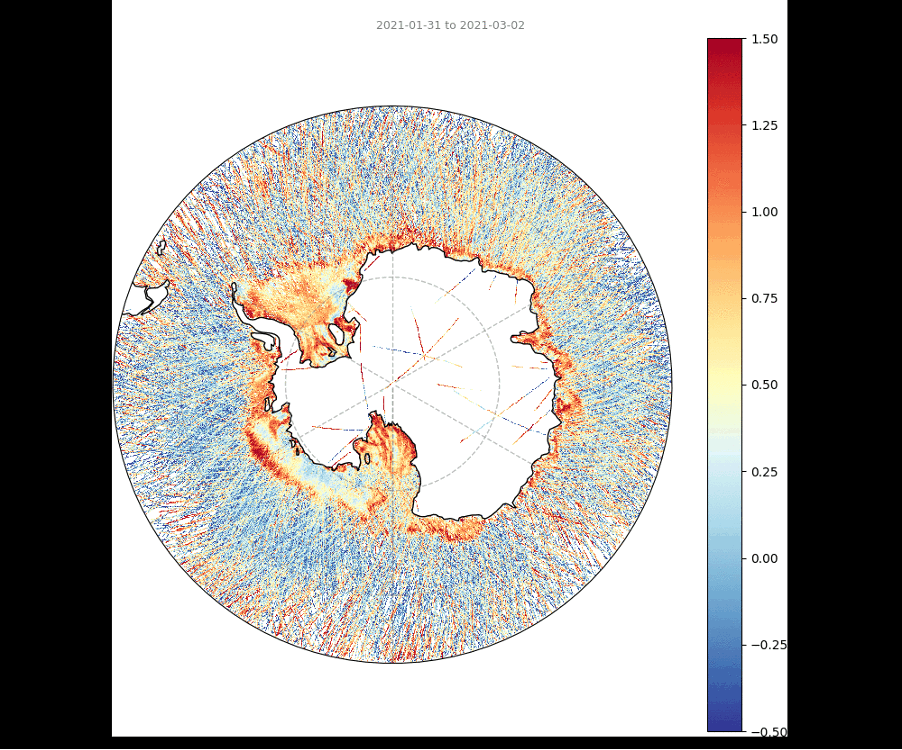
GNSS-R
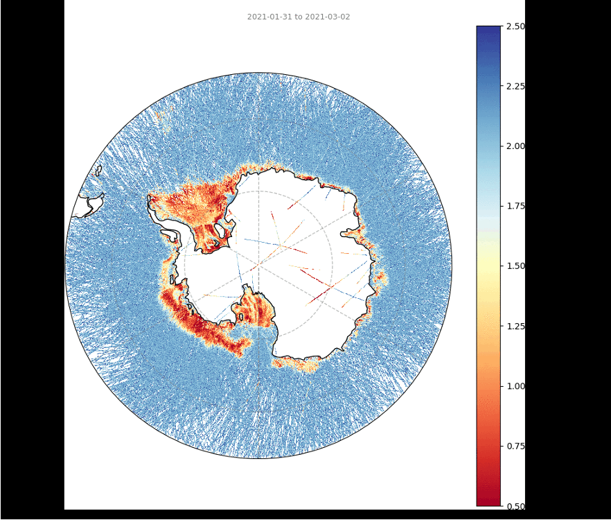
GNSS-R
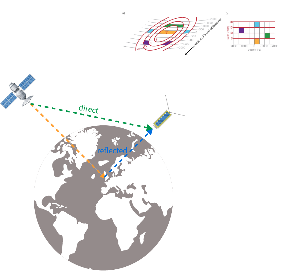
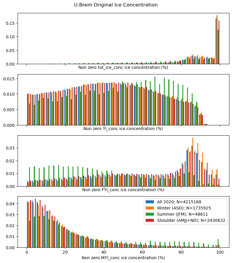
IUP Multiyear ice concentration and other sea ice types, Version AQ2 (Antarctic)
- Provides YI, FYI and MYI concentrations
- Developed by Institute of Environmental Physics, University of Bremen
- Uses passive microwave (AMSR2) and scatterometer (ASCAT instruments on Metop A/B/C) data to derive initial estimates
- Corrects the initial estimates using 2m surface air temperature and sea ice drift data
- 12.5km x 12.5km grid resolution
Melsheimer, Christian; Spreen, Gunnar; Ye, Yufang; Shokr, Mohammed (2019): Multiyear Ice Concentration, Antarctic, 12.5 km grid, cold seasons 2013-2018 (from satellite). PANGAEA, https://doi.org/10.1594/PANGAEA.909054
Sea Ice Signal in GNSS-R features?
Some details
- PCA data:
- water - total ice concentration = 0%
- ice - total ice concentration > 99%
- PCA features:
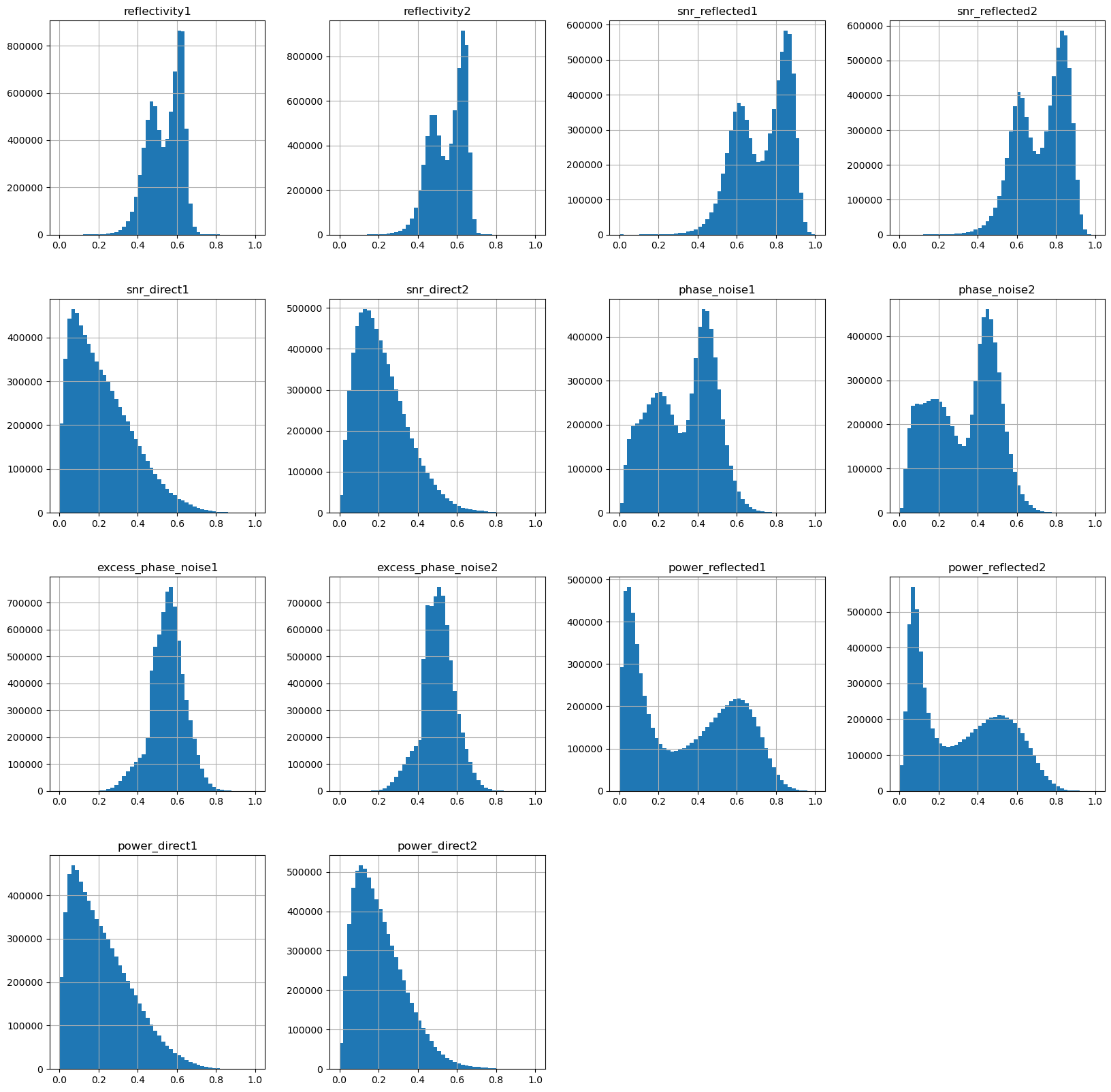
- reflectivity1
- snr_reflected1
- power_reflected1
- phase_noise1
- excess_phase_noise1
- total explained variance: 99.25%
Some details
- PCA data:
- YI - YI ice concentration > 90%
- FYI - FYI ice concentration > 99.9%
- MYI - MYI ice concentration > 99%
- PCA features:
- reflectivity1
- snr_reflected1
- power_reflected1
- phase_noise1
- excess_phase_noise1
- total explained variance: 99.58%
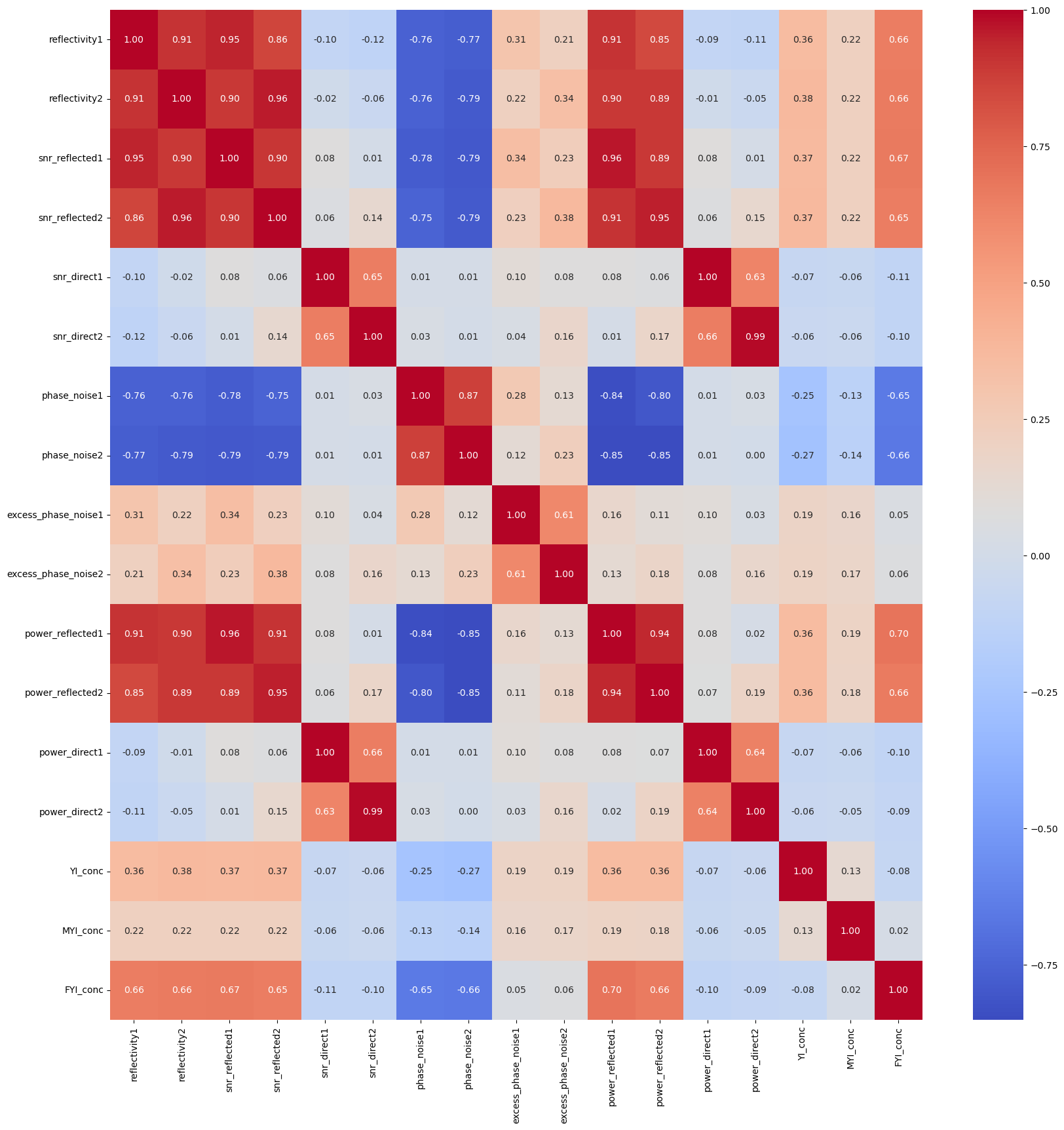
Correlation amongst GNSS-R features and ice types
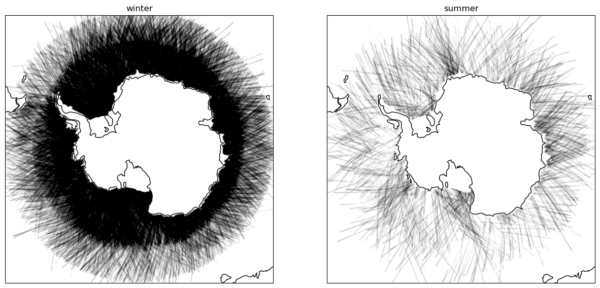
Geographic distribution
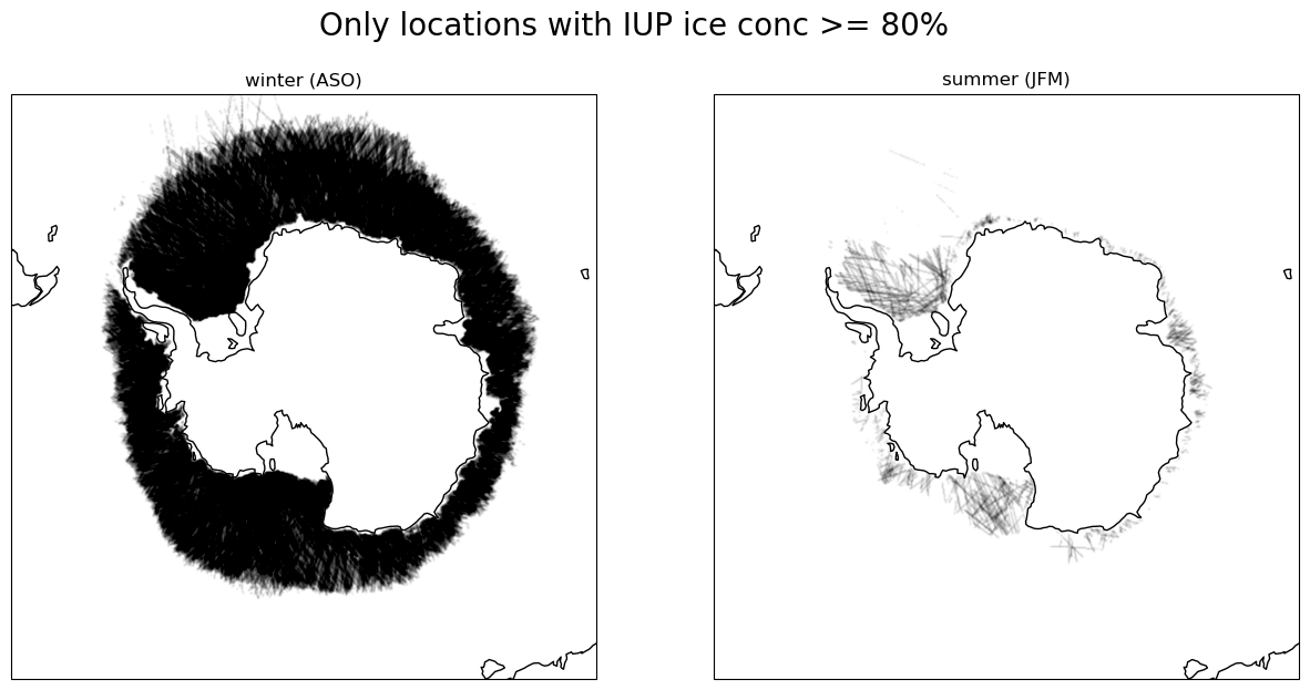
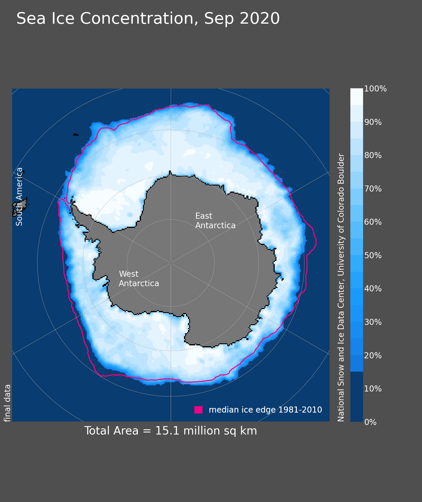
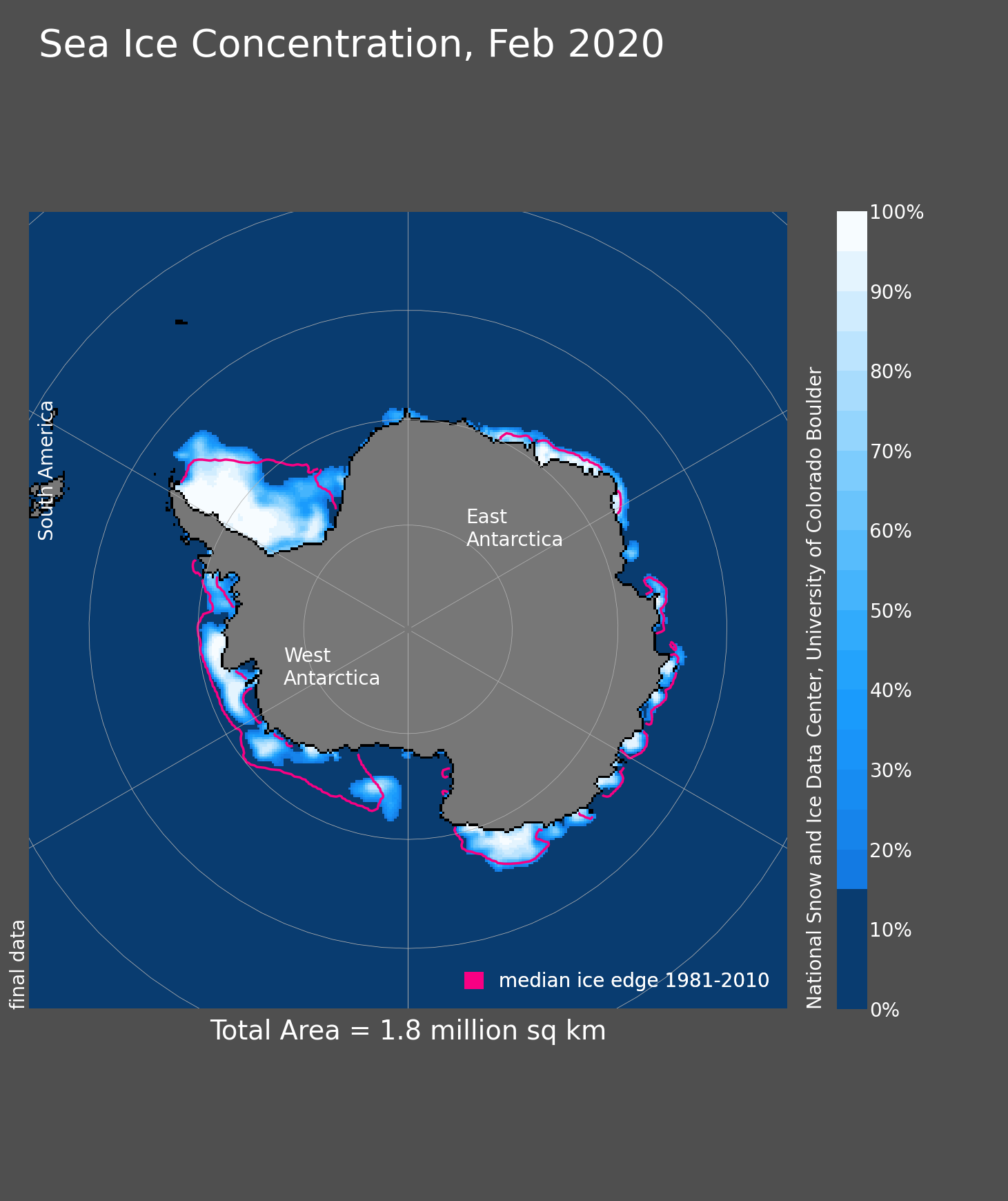
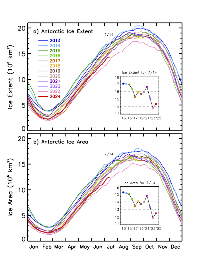
National Snow and Ice Data Center, Boulder, Colorado USA. https://nsidc.org/data/seaice_index, last access: 2024-07-16
J. C. Comiso, A. C. Bliss, R. Gersten, C. L. Parkinson, and T. Markus (2024), Current State of Sea Ice Cover, https://earth.gsfc.nasa.gov/cryo/data/current-state-sea-ice-cover, last access: 2024-07-16.
Ice concentrations as probabilities
- the spatial footprint of GNSS-R grid is around 2.5% of the size of the IUP grid
- interprit ice concentration as the probabiliy of seeing that kind of ice inside that grid
- assume that the ice concentrations can be erroneous
- assume higher ice concentrations are more likely to be correct
- semi-supervised approach: learn a mapping from GNSS-R to ice labels where IUP concentrations are close to 100%
- update the IUP concentrations using the learned mapping
Bayesian update
Two ways to get $P(model\ pred\ |\ true\ label)$:
- Using a tabular ML model - model calibration required
- calibrate using test dataset and Bayes rule again
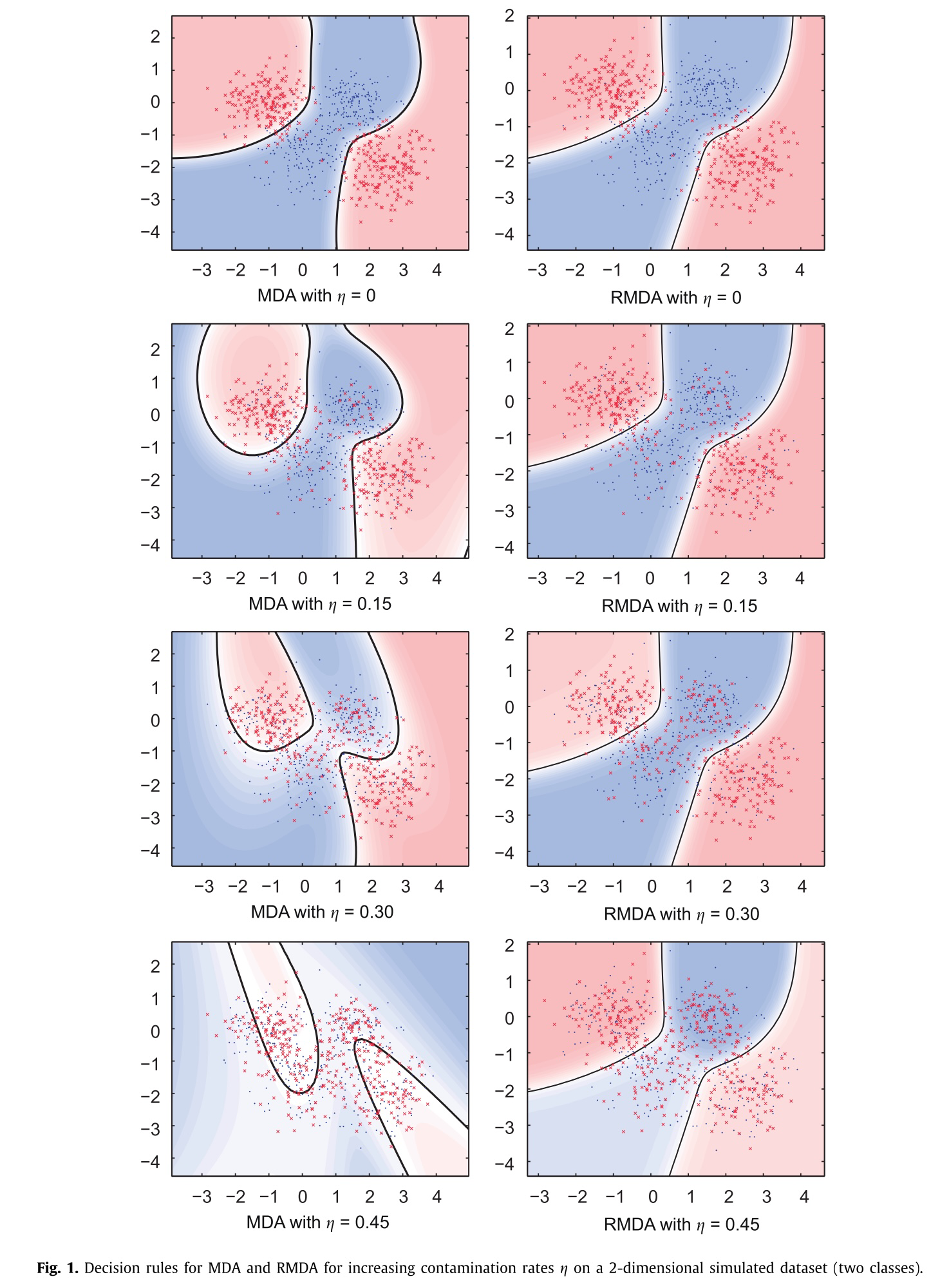
- Using Robust Mixture Discriminent Analysis (RMDA)
Bouveyron, C., & Girard, S. (2009). Robust supervised classification with mixture models: Learning from data with uncertain labels. Pattern Recognition, 42(11), 2649–2658. https://doi.org/10.1016/j.patcog.2009.03.027
Which ML model?
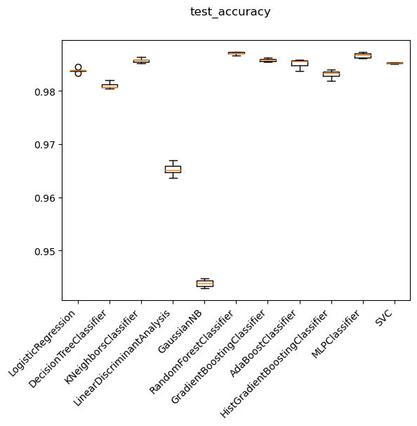
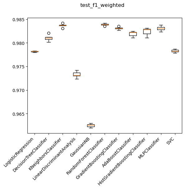
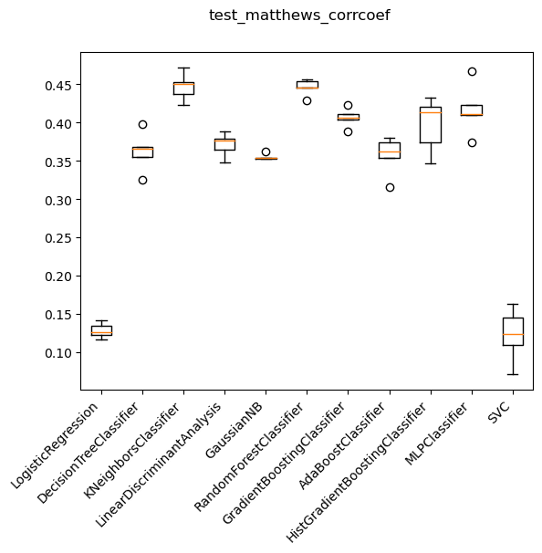
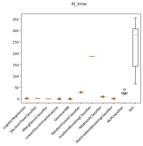
Decision tree ensemble methods
- Random Forest: Fits an ensemble of N trees on random subsets (known as bagging) of data and predicts with a majority vote.
- Adaptive Gradient Boosting: Trains N trees sequentially, each tree correcting the errors of the previous tree by weighting the data points that were misclassified. This is known as boosting.
- Gradient Boosting: Also a boosting method in that it trains N trees sequentially, however, instead of weighting the data points, it fits each tree to the residuals of the previous tree.
LightGBM
Key improvements over vanilla gradient boosting:
- Histogram-based splitting: LightGBM bins the data points into discrete bins and then splits the bins instead of the data points. This reduces the complexity of the model and speeds up training.
- Leaf-wise growth: Instead of growing the tree level-wise, LightGBM grows the tree leaf-wise. This reduces the number of nodes in the tree and hence the complexity of the model.
- Gradient-based One-Side Sampling: LightGBM samples the data points based on the gradient of the loss function. This speeds up training by focusing on the data points that are more informative.
- Exclusive Feature Bundling: LightGBM bundles exclusive features together to reduce the number of features that need to be considered during training.
Gaussian Mixture Discriminant Analysis
Robust Mixture Discriminant Analysis
Class rebalancing
- Training score: 83.7%
- Validation score: 81.3%
| YI | FYI | MYI | water | |
|---|---|---|---|---|
| YI | 0.59237875 | 0.27944573 | 0.0369515 | 0.09122402 |
| FYI | 0.02884615 | 0.94346154 | 0.01884615 | 0.00884615 |
| MYI | 0.08886389 | 0.64904387 | 0.22497188 | 0.03712036 |
| water | 0.02849003 | 0.01745014 | 0.00747863 | 0.9465812 |
- The entire dataset contains 7.39M rows.
- After filtering rows where we have high confidence in labels (YI>90%, FYI>99.9%, MYI>99.%,Water=100%), we are left with:
- YI: 9801 rows
- FYI: 28266 rows
- MYI: 9805 rows
- Water: 3.18M rows
Solution: SMOTE based class rebalancing
SMOTE
- Synthetic Minority Over-sampling Technique
- Identify the minority class
- Find its nearest neighbours
- Generate synthetic samples by interpolating between the minority class and its neighbours
- After SMOTE each class contains 3.18M rows
- So we randomly undersampled and treated the number of samples in each class as a hyperparameter
- More sophisticated undersampling techniques (Tomek, Edited Nearest Neighbours) did not prune the dataset enough
Performance after class rebalancing
| Number of resampled rows in each class | ~1.6M |
| Training accuracy | 99.34% |
| Validation accuracy | 99.12% |
| Test accuracy | 96.34% |
Test Confusion matrix
| YI | FYI | MYI | water | |
|---|---|---|---|---|
| YI | 0.67241379 | 0.15922921 | 0.04158215 | 0.12677485 |
| FYI | 0.04790419 | 0.84677703 | 0.08559352 | 0.01972526 |
| MYI | 0.046875 | 0.25878906 | 0.64257812 | 0.05175781 |
| water | 0.01741254 | 0.00994283 | 0.00626461 | 0.96638002 |
Updated ice probability density
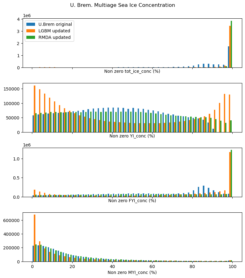
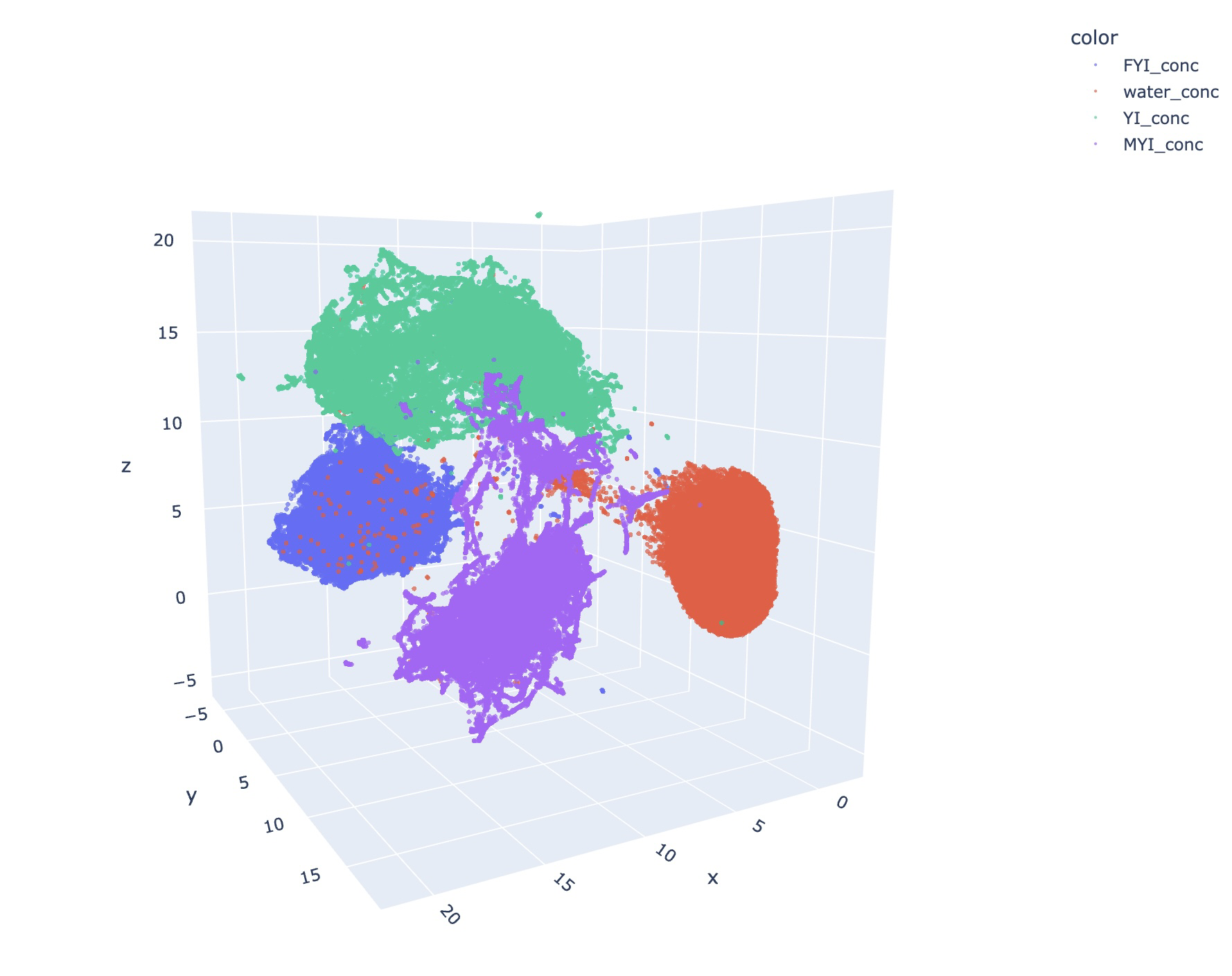
UMAP (Uniform Manifold Approximation and Projection)
- UMAP is a non-linear dimensionality reduction technique that is particularly well-suited for visualizing complex data in a low-dimensional space
- UMAP assumes that high-dimensional data lies on a low-dimensional manifold embedded in the higher-dimensional space
- UMAP first constructs a weighted k-nearest neighbor graph from the high-dimensional data
- UMAP then defines a low-dimensional representation and uses stochastic gradient descent to optimize the layout of the low-dimensional points, preserving the structure of the high-dimensional graph as closely as possible
- It thus preserves both local and global structure of the data
- Supervised mode:
- During knn graph construction, UMAP uses the labels to weight the edges in the graph so that points with the same label are closer in the low-dimensional space
- Also adds a loss term to the optimization function that penalizes points with the same label being far apart in the low-dimensional space
Performance after UMAP feature transformation
| Number of resampled rows in each class | ~300K |
| Training accuracy | 99.99% |
| Validation accuracy | 99.84% |
| Test accuracy | 93.34% |
Test Confusion matrix
| YI | FYI | MYI | water | |
|---|---|---|---|---|
| YI | 0.95866935 | 0.02116935 | 0.0141129 | 0.00604839 |
| FYI | 0.01243201 | 0.95648796 | 0.02175602 | 0.00932401 |
| MYI | 0.01208459 | 0.02819738 | 0.95166163 | 0.00805639 |
| water | 0.04524251 | 0.00951845 | 0.02106578 | 0.92417327 |
Updated ice probability density
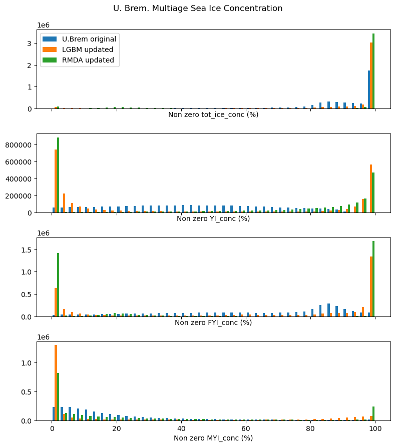
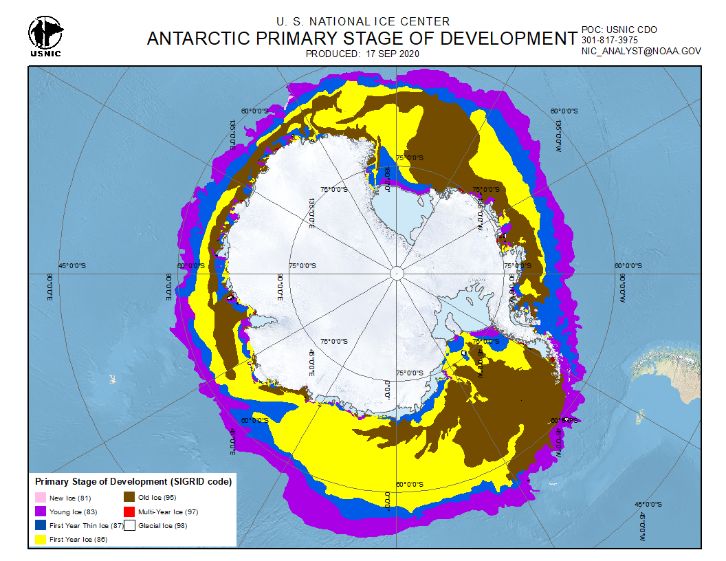
Updated geographic distribution - winter


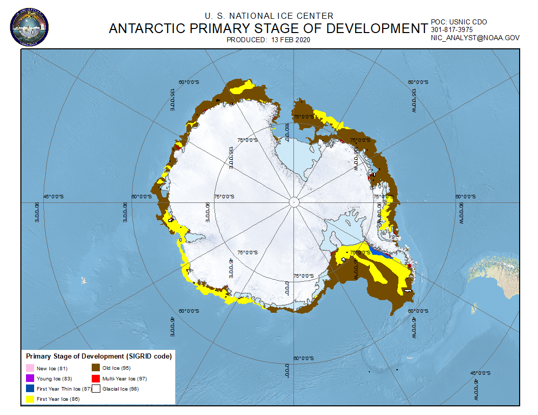
Updated geographic distribution - summer


- GNSS-R is an exciting new data source for monitoring sea ice at very high resolution
- we fitted models to predict ice types and used these models to update existing ice concentration datasets
- we pick up many more locations previously missed thus improving existing ice concentration datasets
- this was only one year of data, the accuracy will improve with more data
More validation required! We are open to ideas